cs180-portfolio

Proj6: NeRF

Exploring stereo correspondence by recreating NeRF.

Part 1: 2D MLP

Basically, for this model, it converts a B x 2 batch of 2D coordinates and then converts it in to a B x 3 batch of rgb values corresponding to those 2D coordinates. That way, I can generate a specifc image from a coordinate system of pixels (important for later). It first takes in the vector $X$. Then, pass it through a Sinusoidal Positional Encoding (SPE) to convert 2D coordinates into 3D coordinates. Then pass the 3D coordinates through a bunch of 256 sized Linear -> ReLU layers. Finally, at the end 3 sized Linear layer, pass the 3d coordinates through a Sigmoid Layer to predict a specific pixel coordinate’s RGB value.

Here’s the architecture for the MLP.

fox.jpg

I initially trained the fox.jpg model with the following parameters: lr=1e-2, num_layers=3, batch_size=10_000, L=10 and iterations=3000. (where lr is learning rate, num_layers is the number of linear/ReLU layers there are, and L being the max frequency for the SPE) I used Mean Squared Error Loss and the ADAM optimizer for training. Furthermore, I also used the Peak Signal-to-Noise Ratio (PSNR) as a measure to determine how “good” an image was.

\[PSNR = 10 \cdot log_{10}\left(\frac{1}{MSE}\right)\]

Here are some images of the the reconstructed image during some of the iterations of the training process with the default hyperparameters:

Iteration 0	Iteration 100	Iteration 200
Iteration 500	Iteration 700	Final

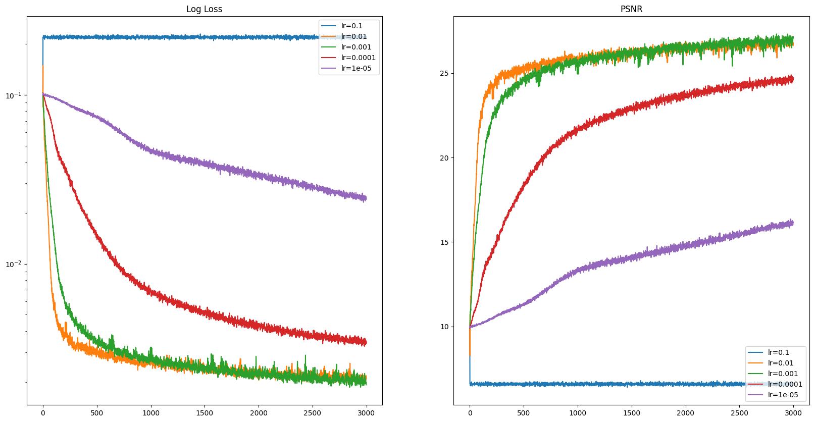
Here are some of the model’s performance after training on varying learning rates and the other hyperparameters remain the same.

Here are some images of the the reconstructed image during some of the iterations of the training process with the default hyperparameters lr=1e-5:

Iteration 0

Iteration 200

Iteration 500

Iteration 700

Final

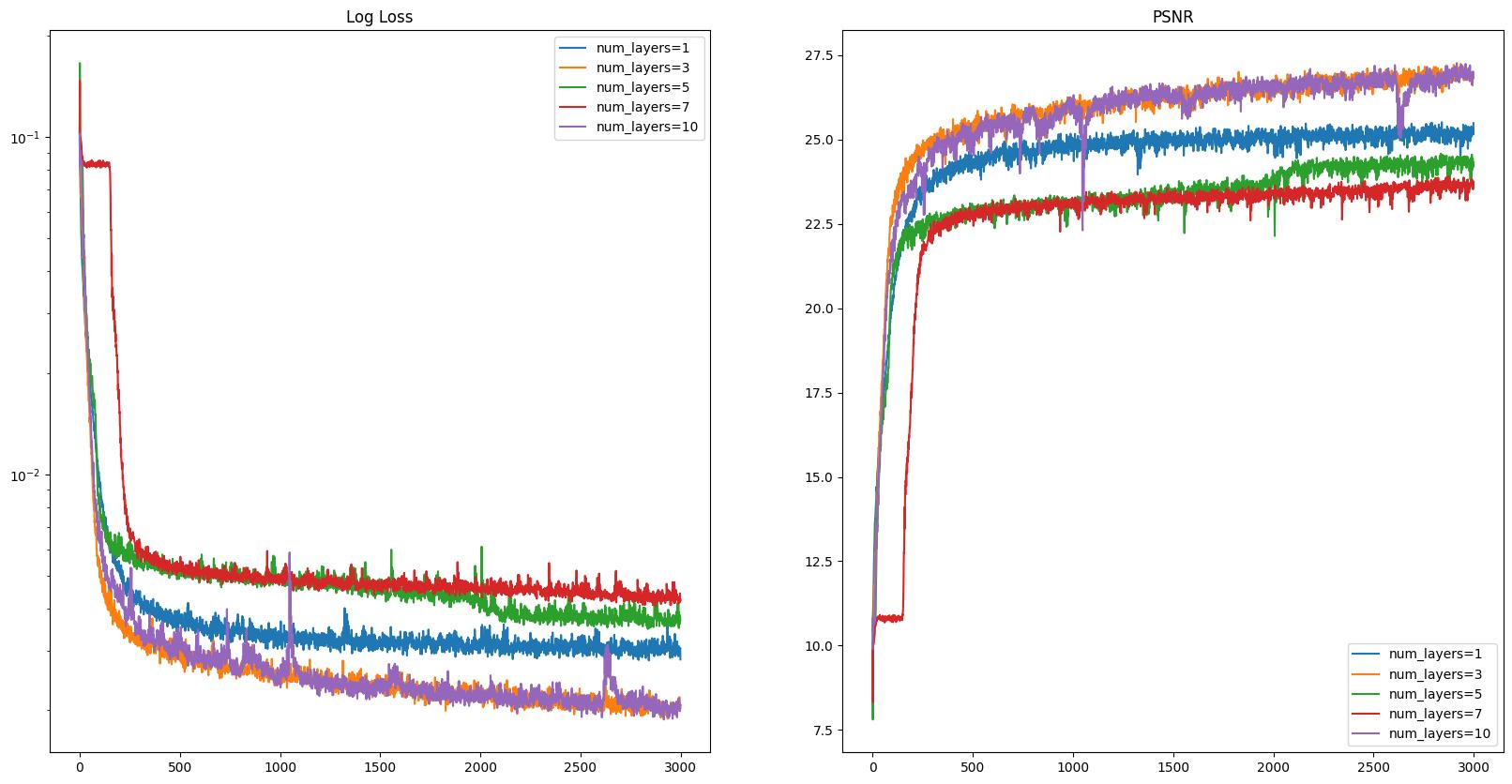
Here are some of the model’s performance after training on varying number of layers in the model and the other hyperparameters remain the same.

Here are some images of the the reconstructed image during some of the iterations of the training process with the default hyperparameters num_layers=7:

Iteration 0	Iteration 100	Iteration 200
Iteration 500	Iteration 700	Final

cat.jpg

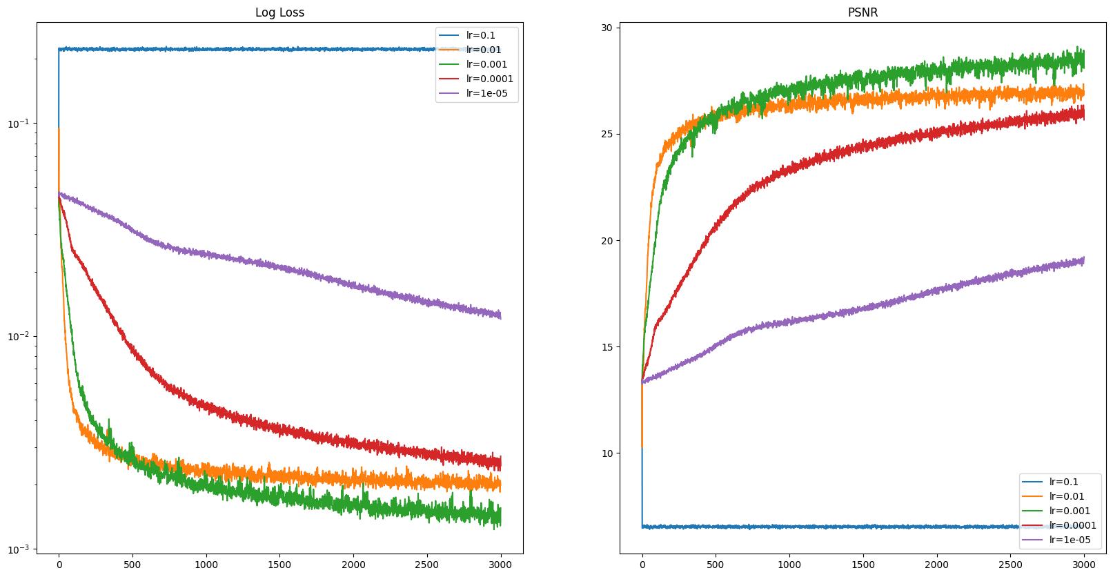
Here’s the MLP network ran with all default parameters and also varying learning rates.

Here’s some iterations of cat.jpg with lr=0.001 (max frequency) and other default hyperparamaters.

Iteration 0	Iteration 100	Iteration 200
Iteration 500	Iteration 700	Final

Part 2: NeRF

transform(c2w, x_c)

I batched transformed 3D camera coordinates x_c into world coordinates using the camera to world c2w transformation matrix. I matrix multiplied by batch using torch.bmm(). This formula is the conversion from world coordinates to image coordinates using the world to camera coordinate transformation matrix w2c. Keep in mind that that coordinates are stored (B, 3) tensors, while the formula is in 3 x 1 vectors for coordinates, so overall,I implemented the transpose of the formula after moving everything to one side by inversing the w2c matrix to get the c2w matrix.

pixel_to_camera(K, uv, s)

Given the focal depth of the camera and the image dimensions, one can create the intrinsic matrix $K$.

$K$ is then used to project a 3D point into the camera coordinate x_c system using 2D pixel coordinates uv of an image. s here is used to provide to the depth to the 2D pixel coordinate so that it can be translated into 3D camera coordinates. Once again, I implemented the transpose of the formula for batched operations so it will be faster.

pixel_to_ray(K, c2w, uv)

Given pixel coordinates, intrinsic matrix $K$, and c2w transformation matrix, we can find the origin of the camera and produce rays that will represent the camera’s line of sight and how a 3D world coordinate is projected onto the image as a pixel from the camera’s point of view.

The origin ray is calculated via this formula, where $R_{3x3}$ and $t$ is from the w2c matrix mentioned above.

\[\begin{align} \mathbf{r}_o = -\mathbf{R}_{3\times3}^{-1}\mathbf{t} \end{align}\]

The distance ray is calculated by this formula, where $X_w$ are world coordinates. The direction array is then noramlized into a unit vector norm using the l2 (or euclidan) norm.

\[\begin{align} \mathbf{r}_d = \frac{\mathbf{X_w} - \mathbf{r}_o}{||\mathbf{X_w} - \mathbf{r}_o||_2} \end{align}\]

Once again, I used torch.bnn() for batched matrix multiplications for faster operations.

Sampling Rays

I created a RaysDataset class that contains all the pixel values and calculate ray values based off of pixel coordinates when sampled. Therfore, the sampling function was also built into this data set with a parameter batch for batch size.

When sampling, I flattened all coordinates of images in the image dataset into a 2D tensor and then used torch.randint to generate a list of random pixels to sample and rays to generate. I then returned a tuple containing (batch, ...) sized tensors of the origin rays ray_o, the direction rays ray_d and the pixel values of said coordinate pixels.

Also all data was normalized for easier computation. i.e. RGB / 255.0

Sampling Plenoptic Points

Now that we have sampled random camera origins and camera directions (corresponding to image pixels), we can now sample points along this ray to get points that are represented by the Plenoptic function. This function is crucial to implement and I had several bugs where the (u, v) coordinates didn’t correspond with the rays, or where (u, v) was flipped to (v, u).

These points along with their direction ray correspondence then can be used to train a MLP deep neural network to output color and density values.

Here are the sampled rays from all cameras.

Here are the sampled rays from one camera

Here are the sampled rays from one camera on the top right from camera pov.

3D MLP Neural Network

I had the model forward function take in (N, n_samples, 3) tensors for both points and direction ray and then flattened the tensors within the forward function such that the Linear Layer can take it as an input. I would then unflatten the tensors after forwarding the inputs through the layers. Lastly, I would unflatten the tensors back into (N, n_samples, _) tesnors and return it. This simplified some processes and made the code looke cleaner

Here’s the structure of the MLP for NeRF.

Volumic Rendering

Using the batched densities and color values predicted by the model, as well as the dt between the n_samples samples along the ray, we can use volumetric rendering to predict a image coordinate pixel’s color values.

We can do so using this discrete approximation of the formula.

\[\begin{align} \hat{C}(\mathbf{r})=\sum_{i=1}^N T_i\left(1-\exp \left(-\sigma_i \delta_i\right)\right) \mathbf{c}_i, \text { where } T_i=\exp \left(-\sum_{j=1}^{i-1} \sigma_j \delta_j\right) \end{align}\]

To implement this in code, I used torch.cumsum to calculated $T_i$ by running getting the cumulative sum of dt * densities and then subtracting densities from that cumsum such that we only get the sum up to i-1. Afterwards, I calculated the main function by multiplying $T_i$ with 1 - torch.exp(-densities * dt) and the colors passed in. Lastly, I summed up the result using torch.sum along the dim=1, to get the sum for each batched image.

Training The Model

The training loop goes as follows:

Sample rays_o, rays_d, pixels
Get the sampled points along rays_d
Pass in points and rays_d through the model’s forward function
Pass in pred_densities and pred_rgb from the model’s output into the volumetric_rendering function
Compare the rgb predicted by volumetric_rendering with the sampled pixels using a loss function
- I used nn.MSELoss
Backpropogate and optimizer takes gradient step

Train Loss and PSNR

I ran 3000 iterations with batch_size=30_000 to achieve 0.004 training loss and 23.435 training PSNR.

Validation Loss and PSNR

I ran 3000 iterations with batch_size=30_000 to achieve 0.003 validation loss and 25.161 validation PSNR.

There is probably something still wrong with my training loop, seeing that validation loss is lower than training loss.

Rendering the Image

Reshape the volumetric_rendering(pred_densities, pred_colors, dt) output into the original images’ dimension to the right corresponding coordinate system.

GPU may run out of memory, so “batch” the rendering process by calculating the predicted rgb values for sections of the image and then concatenating the results afterwards. Be careful to only transpose the image after concatenating everything. I personally did the reconstruction in 200x20 batches.

Validation Image Reconstruction

These are reconstructions of the 0th image of the validation set during different iterations of the training process.

Iteration 0	Iteration 100	Iteration 200
Iteration 500	Iteration 700	Iteration 900
Iteration 3000	Iteration 3500	Iteration 3900

Running NeRF on `c2w` Test Set

Given a bunch of camera to world coordinate transformation matrices, the model generates the lego CAT.

Bells and Whistles

Depth Perception

This was done by modifying the volumetric perceptron function a bit. Instead of multiplying the equation with predicted rgbs, multiply the equation with torch.linspace(1, 0, n_samples) to put a near to far weight on the densities on a particular ray direction. Lighter is closer, darker is further.

proj6: reflection

I learned a lot on how NeRF works through this project. It was fun yet tough to implement, but I did learn more about stereo correspondence and plenoptic functions. I think I can also increase my PSNR by changing my model architecture to be Tensored based rather than MLP according to this paper. I think it is pretty interesting and I probably look into other different architectures and methods to increase PSNR.

back to project list